Panorama Stitching from Scratch
When you sweep your phone across a skyline in panorama mode, the result is a single seamless, ultra-wide photograph. The process behind it can feel like magic - but it is roughly 150 lines of Python, and by the end of this post you will have seen all of them work.
Our task: take these two photos of the University of Colorado Boulder campus, with the Flatiron mountains behind, shot from the same position but with the camera rotated between shots (and, as often happens with auto-exposure, with slightly different brightness):
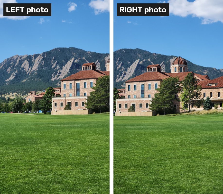
1. Why the naive approach fails
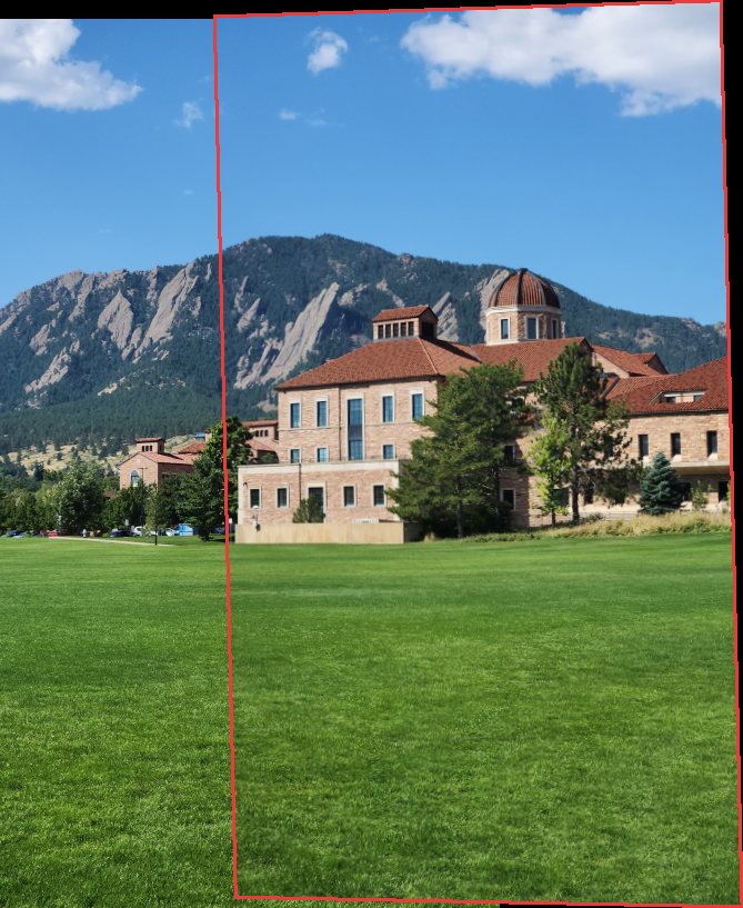
A tempting first idea: slide the right photo horizontally until it lines up, then average the overlap.
Here is that plan, executed exactly:
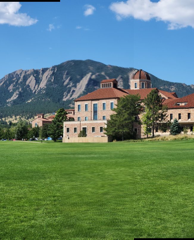
Two problems, both fatal:
- Geometry. The camera rotated between shots, so the right photo isn’t just shifted - it’s rotated and slightly keystoned. No amount of sliding fixes that. We need a warp.
- Photometry. The two photos have different brightness (auto-exposure did that), so even where they do line up, you can see the seam.
The real pipeline fixes both:
- Find corners in each image (Harris)
- Spread them out across the image (ANMS)
- Describe each corner with a compact numeric signature
- Match descriptors across the two images
- Reject false matches (RANSAC) and fit a homography
- Warp one image onto the other
- Blend away the seam
Every step below follows the same rhythm: intuition → code → result, plus something you can poke at. All the code runs with just numpy and opencv-python, and every piece of it appears in the sections below.
import cv2
import numpy as np

im1 = cv2.imread("left.jpg")          # 450 x 800
im2 = cv2.imread("right.jpg")
g1 = cv2.cvtColor(im1, cv2.COLOR_BGR2GRAY).astype(np.float32)
g2 = cv2.cvtColor(im2, cv2.COLOR_BGR2GRAY).astype(np.float32)
2. Detecting corners (Harris)
To align two images, we need landmarks that we can find in both - distinctive points we could recognize again. What makes a point recognizable?
Imagine sliding a tiny window around the image and asking: “if I nudge this window a little, does what’s inside change?”
- On flat sky: shift it anywhere and nothing changes. A patch of sky could match countless other patches of sky, so it is useless as a landmark.
- On an edge: shift it along the edge and nothing changes; shift it across and everything changes. Only half-useful - the point can be localized in one direction only.
- On a corner: shift it in any direction and the content changes. A corner is pinned down in both and .
The Harris corner detector turns this into math. Around each pixel, collect the image gradients over a small window and build the structure tensor
The two eigenvalues of measure “how much the patch changes” along the two principal directions: both small → flat, one large → edge, both large → corner. Rather than computing eigenvalues explicitly, Harris uses the famous shortcut score
which is large and positive at corners, negative on edges, and near zero in flat regions. OpenCV does the sliding-window part for us; we keep every pixel that beats its 8 neighbours, so each corner is counted once rather than dozens of times:
def harris_corners(gray):
    R = cv2.cornerHarris(gray, blockSize=2, ksize=3, k=0.04)
    R_dilated = cv2.dilate(R, None)          # 3x3 local max filter
    is_peak = (R == R_dilated) & (R > 1e-4 * R.max())
    ys, xs = np.nonzero(is_peak)
    scores = R[ys, xs]
    order = np.argsort(-scores)              # strongest first
    return np.column_stack([xs, ys])[order], scores[order]

pts1, sc1 = harris_corners(g1)   # ~11,000 candidate corners
pts2, sc2 = harris_corners(g2)
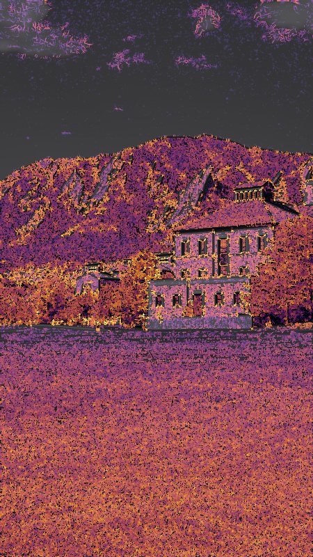
Here is the Harris response over the left photo - brighter means a stronger corner score:
And thresholding + keeping local peaks gives us actual points:
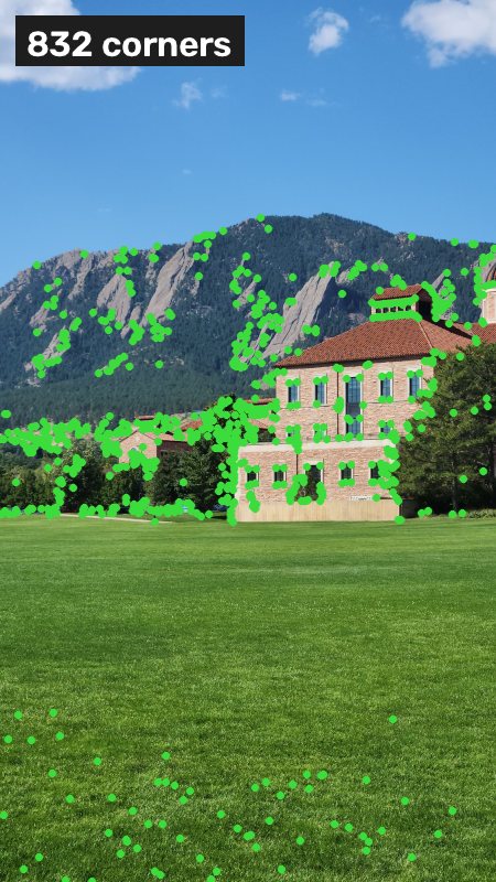
Try setting the threshold yourself. Drag the slider and observe the trade-off: too lenient and noise floods in; too strict and only a handful of very strong corners survive:
Quick check: why does the sky have (almost) no corners, while the lawn has many weak ones?
The sky is textureless - slide a window anywhere and it sees the same blue, so both eigenvalues are tiny and R ≈ 0. The lawn does have fine texture (blades of grass, mowing stripes), so it produces plenty of corners - but they are weak and all look nearly identical. Keep that in mind; those repetitive grass corners will cause trouble in the matching step.
3. Spreading corners across the image (ANMS)
We have ~11,000 corners per image but only need a few hundred. The obvious selection - keep the strongest - turns out to be a mistake.
The problem is that corner strength is spatially clumped. The stone facade and the treeline generate hundreds of very strong corners in one band of the image, so “top 300 by strength” yields 300 points crowded there and almost nothing elsewhere:
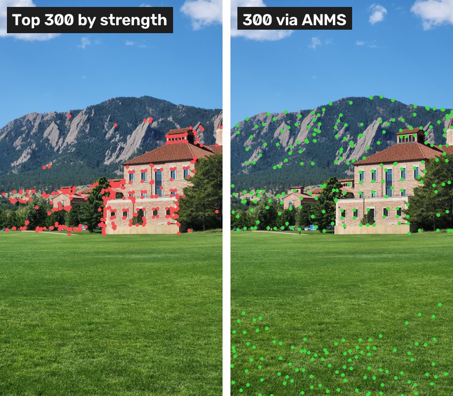
Why is clumping bad? Because we will fit a warp for the whole image from these points, and estimating a global transform from points concentrated in one small region is like polling a single neighborhood and calling it a national survey.
Adaptive Non-Maximal Suppression (ANMS) fixes it with one elegant idea: for each corner , ask
“How far away is the nearest corner that is meaningfully stronger than me?”
Call the corner’s suppression radius. A corner with a large radius dominates a large neighbourhood - those are worth keeping. A strong corner sitting next to an even stronger one has a tiny radius and can be dropped. Then “keep corners” simply means “keep the largest radii”, and spatial coverage follows automatically. (The factor means a corner is only suppressed by neighbours at least 10% stronger - it prevents two nearly-tied neighbours from suppressing each other arbitrarily.)
def anms(pts, scores, num_keep=500, c_robust=0.9):
    pts = pts[:1200].astype(np.float64)      # only consider the strongest 1200
    scores = scores[:1200]
    # d2[i, j] = squared distance from corner i to corner j
    d2 = ((pts[:, None, :] - pts[None, :, :]) ** 2).sum(axis=2)
    # only distances to corners that are meaningfully stronger count
    meaningfully_stronger = scores[None, :] * c_robust > scores[:, None]
    d2 = np.where(meaningfully_stronger, d2, np.inf)
    radius = np.sqrt(d2.min(axis=1))         # suppression radius per corner
    radius[0] = np.inf                       # the strongest corner fears no one
    return pts[np.argsort(-radius)[:num_keep]]

keep1 = anms(pts1, sc1)   # 500 well-spread corners, left image
keep2 = anms(pts2, sc2)
Toggle between the two strategies and vary N. Note where the red points land compared to the green ones:
To experiment with the algorithm directly, here is ANMS on a synthetic “corner map” with two strength hotspots - run it, then try changing N or the hotspot sizes:
ANMS playground (editable)
Quick check: the single strongest corner gets radius = ∞. Why?
Its suppression radius is “distance to the nearest stronger corner” - and no stronger corner exists. Nothing can suppress it, so it is always kept, no matter how small N is.
4. Describing corners
We have 500 corners in each image. Now, for each corner in the left image, we need to find the same physical point among the right image’s corners. To compare corners, each one needs a descriptor - a compact numeric signature of what the image looks like around it.
The simplest idea is to take the 40×40 pixel patch around the corner and use it directly. Almost - but raw patches are too literal. If the corner’s position is off by two pixels (it will be) or the exposure differs (ours does), raw patches disagree everywhere. So we deliberately coarsen them:
- Blur the patch (Gaussian, ) - small misalignments stop mattering.
- Shrink 40×40 → 8×8 - keeps the gist, discards fragile detail. 64 numbers.
- Normalize to zero mean and unit variance - the key step: for a patch , use , and brightness shifts and contrast changes vanish. A dark version and a bright version of the same patch become the same descriptor.
def make_descriptors(gray, pts, patch=40, out=8):
    blurred = cv2.GaussianBlur(gray, (0, 0), 2.5)
    h, w = gray.shape
    descriptors, kept_pts = [], []
    for x, y in pts.astype(int):
        if not (patch//2 <= x < w - patch//2 and patch//2 <= y < h - patch//2):
            continue                          # too close to the border
        p = blurred[y - patch//2 : y + patch//2, x - patch//2 : x + patch//2]
        p = cv2.resize(p, (out, out), interpolation=cv2.INTER_AREA).ravel()
        p = (p - p.mean()) / (p.std() + 1e-8)   # exposure-proof!
        descriptors.append(p)
        kept_pts.append((x, y))
    return np.float32(descriptors), np.float64(kept_pts)

D1, kp1 = make_descriptors(g1, keep1)
D2, kp2 = make_descriptors(g2, keep2)
Here is what three corners look like as they go from context → 40×40 patch → 8×8 descriptor:
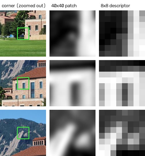
Quick check: our two photos came out with slightly different exposure. Which of the three steps handles this, and how?
Normalization. Subtracting the mean cancels any brightness offset; dividing by the standard deviation cancels contrast scaling. A patch and its darker twin map to identical descriptors - so matching is unaffected by the exposure difference. (Blending will still have to deal with it later, though.)
5. Matching descriptors
Time to match. For every left descriptor, compute its distance to every right descriptor (64-dimensional sum of squared differences), and note the best and second-best candidates.
Now the crucial question: when is a match trustworthy? Not simply when the best distance is small - repetitive structures (windows, railings, ripples) produce many small distances. The real signal is when the best match is much better than the runner-up:
This is David Lowe’s ratio test: a match that is only marginally better than its runner-up is probably a guess, and should be discarded.
d2 = ((D1**2).sum(1)[:, None] + (D2**2).sum(1)[None, :] - 2 * D1 @ D2.T)
nearest2 = np.argsort(d2, axis=1)[:, :2]           # best & runner-up per row
best  = d2[np.arange(len(D1)), nearest2[:, 0]]
runup = d2[np.arange(len(D1)), nearest2[:, 1]]
ratio = np.sqrt(best / runup)                      # 0 = confident, 1 = coin flip

is_match = ratio < 0.8
match_p1 = kp1[is_match]                           # left points
match_p2 = kp2[nearest2[is_match, 0]]              # their right partners
With ratio < 0.8 we get 190 matches:
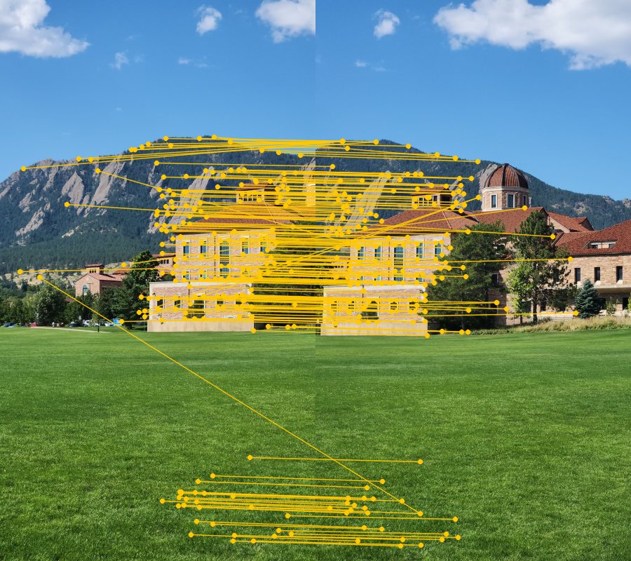
Try it yourself. Loosen the ratio threshold and watch unreliable matches flood in; then enable “reveal outliers” to see which matches were actually correct (using the answer computed in the next section):
Quick check: why compare best vs. second-best instead of just thresholding the best distance?
Because “small distance” means different things in different places. On unique structure, even the best match has a moderate distance; on repetitive texture (dozens of identical windows, shimmering water), many candidates have tiny distances. An absolute threshold cannot serve both. The ratio asks “is this match uniquely good?”, which is exactly the property we need - a match that is barely better than its runner-up is probably a guess.
6. Interlude: the transformation we are estimating (homographies)
Before we can reject the false matches, we need to know what the correct matches agree on. What is the actual geometric relationship between the two photos?
When a camera rotates in place (your arm doing the pano wave), the two images are related by a homography: a 3×3 matrix that maps every pixel of one image to its position in the other, in homogeneous coordinates:
That divide-by- is what makes a homography more powerful than rotate+shift: it can make parallel lines converge - the keystone “leaning building” effect - which is exactly what camera rotation does to the world.
has 8 unknowns (). Each match pins down 2 equations (one for , one for ), so 4 matches determine a homography. Given 4+ matches, we build a linear system and solve for the null space with SVD - the classic Direct Linear Transform (DLT). The code is short (production implementations also normalize the coordinates before solving, which improves numerical stability):
def apply_h(H, pts):
    """Apply H to Nx2 points, including the divide-by-w'."""
    p = np.column_stack([pts, np.ones(len(pts))]) @ H.T
    return p[:, :2] / p[:, 2:3]

def dlt_homography(src, dst):
    """Fit H such that dst ~ H @ src, from N >= 4 point pairs."""
    A = []
    for (x, y), (u, v) in zip(src, dst):
        A.append([-x, -y, -1,  0,  0,  0, u*x, u*y, u])
        A.append([ 0,  0,  0, -x, -y, -1, v*x, v*y, v])
    _, _, Vt = np.linalg.svd(np.array(A))
    H = Vt[-1].reshape(3, 3)      # null space = the h that makes A @ h ~ 0
    return H / H[2, 2]
So: 4 good matches determine the warp exactly. But give DLT even one false match and it will produce a badly wrong estimate. With a meaningful fraction of our matches being false, least-squares over everything is hopeless. We need an estimator that is robust to outliers.
7. Robust fitting with RANSAC
RANSAC (RAndom SAmple Consensus) solves this with a voting scheme:
- Pick 4 matches at random. Fit a homography to just those 4.
- Ask every match to vote: warp your left point with - does it land within 4 pixels of your right point? If yes, you’re an inlier for this .
- Count votes. Remember the with the most.
- Repeat a few hundred times. Finally, refit using all inliers of the winner - a big, stable least-squares, now safe because the liars are gone.
Why it works: false matches are essentially random - they do not agree with each other. Correct matches all agree on the one true warp. So the moment a random sample happens to contain 4 correct matches, all of the correct matches vote yes at once, and no subset of outliers can ever reach a comparable score.
best_inliers = None
for _ in range(600):
    sample = np.random.choice(len(match_p1), 4, replace=False)
    H = dlt_homography(match_p2[sample], match_p1[sample])
    projected = apply_h(H, match_p2)                  # warp right pts to left frame
    err = np.linalg.norm(projected - match_p1, axis=1)
    inliers = err < 4.0                               # pixels
    if best_inliers is None or inliers.sum() > best_inliers.sum():
        best_inliers = inliers

H = dlt_homography(match_p2[best_inliers], match_p1[best_inliers])  # final refit
The verdict on our 190 matches - 168 inliers (green), 22 outliers (red):
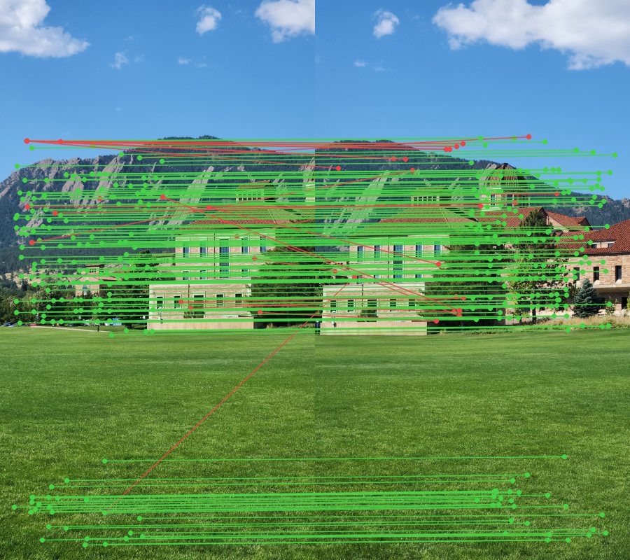
Run the sampling yourself. Each iteration picks 4 random matches, fits , and counts the votes. Note how a single outlier in the sample collapses the vote count - and how good iterations all agree on roughly the same consensus:
How many iterations do we need? If a fraction of matches are correct, one sample of 4 is all-correct with probability , so after iterations
With our : one sample is clean with probability , and the failure probability after just 10 iterations is about . That is the key insight of RANSAC - you do not need most samples to be good, you need one, and one arrives quickly. (Real systems solve this formula backwards to pick the number of iterations.)
RANSAC applies far beyond panoramas - it protects any model-fitting from outliers. Here it is applied to a simple line fit; run it, then increase N_OUTLIERS and compare how least squares and RANSAC degrade:
RANSAC vs. least squares (editable)
8. Warping
We have . Now we use it: warp the right image into the left image’s coordinate frame and place both on a shared canvas.
One subtlety worth knowing - warping runs backwards. Instead of pushing each right-image pixel to its new home (which leaves holes), we go through every pixel of the output, apply to ask “where in the right image does this come from?”, and sample there. cv2.warpPerspective does this for us. We just have to compute a canvas big enough to hold both images: warp the 4 corners of the right image, take the bounding box, and shift everything by a translation so nothing lands at negative coordinates.
corners = np.float64([[0, 0], [W, 0], [W, H_img], [0, H_img]])
warped_corners = apply_h(H, corners)
x0, y0 = np.floor(np.minimum(warped_corners.min(0), 0)).astype(int)
x1, y1 = np.ceil(np.maximum(warped_corners.max(0), [W, H_img])).astype(int)
T = np.array([[1, 0, -x0], [0, 1, -y0], [0, 0, 1.0]])   # keep pixels positive

canvas_size = (x1 - x0, y1 - y0)
warped2 = cv2.warpPerspective(im2, T @ H, canvas_size)
canvas1 = np.zeros_like(warped2); canvas1[-y0:-y0+H_img, -x0:-x0+W] = im1
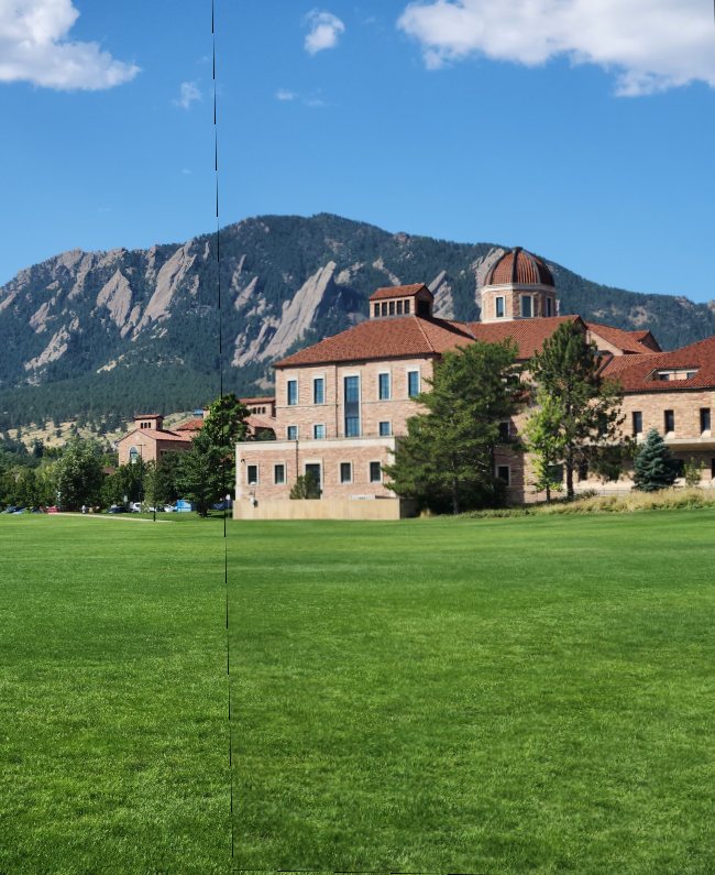
Geometrically, this works very well - the roofline, the stone facade and the mountain ridge continue smoothly through the boundary. But paste one image over the other and the junction is still visible:
9. Blending the seam
The remaining artifact is the seam itself. The classic fix is feathering: in the overlap, cross-fade between the images - weighted intelligently. Each pixel gets a weight equal to its distance to the edge of its own image (a distance transform gives us this in one call), so an image contributes little near its own border and dominates deep inside its own region:
def feather_weight(mask):
    return cv2.distanceTransform(mask.astype(np.uint8), cv2.DIST_L2, 5)

w1 = feather_weight(mask1)                # mask1/mask2 = where each image has pixels
w2 = feather_weight(mask2)
total = np.maximum(w1 + w2, 1e-6)
panorama = (canvas1 * (w1/total)[..., None] +
            warped2 * (w2/total)[..., None]).astype(np.uint8)
The seam region, before and after:
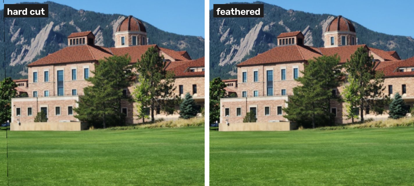
Drag the divider - left of the line is the hard cut, right of it is the feathered blend:
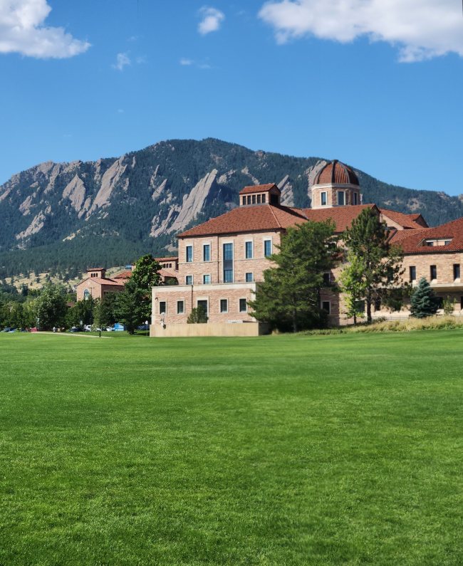
And with that, the finished panorama - two photographs in, one wide image out:
10. Summary
The whole pipeline in one paragraph: Harris found thousands of recognizable points; ANMS kept 500 well-spread ones; blurred, downsampled, normalized descriptors made them comparable across exposure changes; the ratio test matched them; RANSAC rejected the 22 outliers; DLT fit the homography from the 168 remaining matches; warpPerspective mapped the right photo into place; and feathering removed the seam.
A useful sanity check: the final homography fits its 168 inliers with a mean reprojection error of about 1 pixel (median 0.8 px) - sub-pixel agreement, estimated from nothing but the pixels themselves.
11. The same pipeline on other scenes
Nothing above is specific to our two campus photos. Here is the identical pipeline, unchanged, on two more sequences from the same dataset.
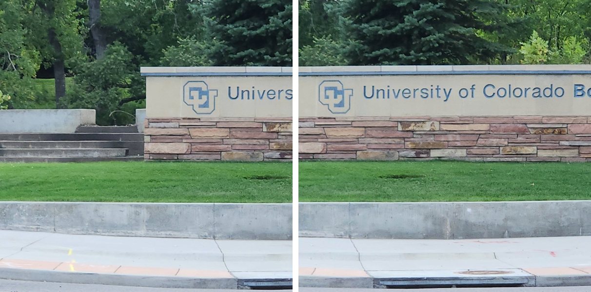
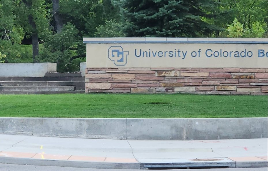
First, two handheld photos of the university’s entrance sign. 206 matches survive the ratio test, RANSAC keeps 162 inliers, and the seam disappears into the stonework:
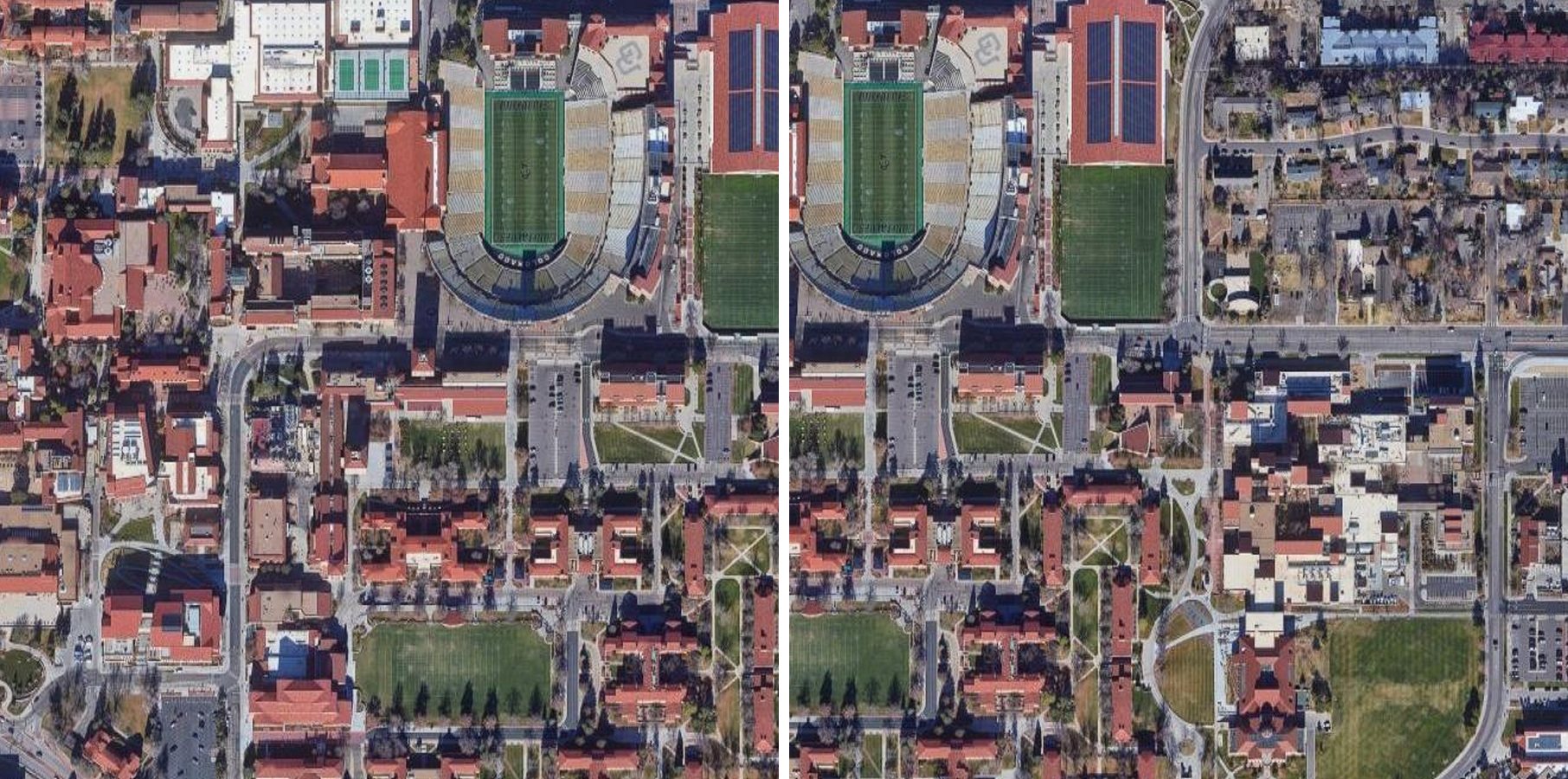
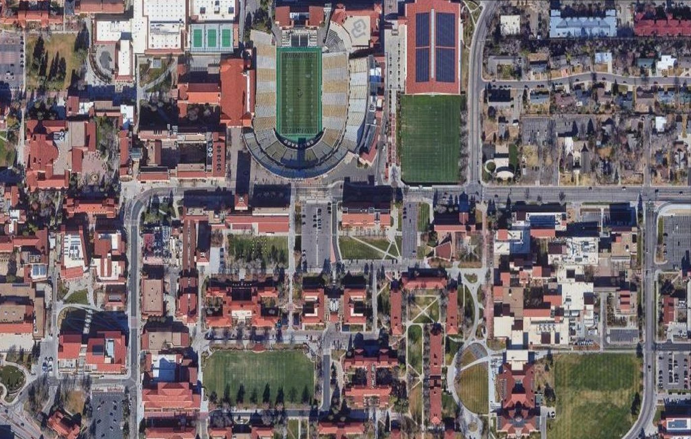
Second, two overlapping aerial tiles of the Boulder campus. A scene viewed from far away is nearly planar, which is the other case a homography models exactly - so the tiles align almost perfectly, with 223 of 253 matches accepted as inliers:
Challenges
- Your own photos. Take two shots out your window (rotate, don’t sidestep - a homography assumes rotation about the camera) and run the pipeline from this post on them.
- Three or more images. The full Flatirons sequence has five photos - stitch neighbours pairwise and chain the homographies onto one canvas. What slowly goes wrong as the chain grows?
- Gain compensation. We hid the exposure difference with feathering; instead, estimate a brightness scale between images from the overlap and correct it before blending.
- Improve the blend. Feathering can ghost when alignment is imperfect - implement two-band (Laplacian pyramid) blending and compare.
- Improve the features. Swap our 8×8 patches for
cv2.SIFT_create()and re-run the pipeline. What survives rotation and zoom now?
Further reading
- Szeliski, Computer Vision: Algorithms and Applications - the image stitching chapter (free online).
- Brown & Lowe, Automatic Panoramic Image Stitching using Invariant Features (2007) - the AutoStitch paper; our pipeline is a simplified version of it (it also introduced this flavor of gain compensation and multi-band blending).
- Harris & Stephens, A Combined Corner and Edge Detector (1988) - the corner classic.
- Lowe, Distinctive Image Features from Scale-Invariant Keypoints (2004) - SIFT and the ratio test.
Photo credit: the input photographs were taken by Chahat Deep Singh on the University of Colorado Boulder campus, with the Flatiron mountains in the background. For a different view of the same mountains, see the Flatirons covered in snow.