Motion Fields and Optical Flow

November 5, 2026

When a camera moves through a scene, each visible 3D point traces a path across the image plane. The motion field is the projection of this 3D motion onto the image: it assigns a 2D velocity to every image point. This post derives the motion field equation and shows what it reveals about scene depth and camera motion.

Setup

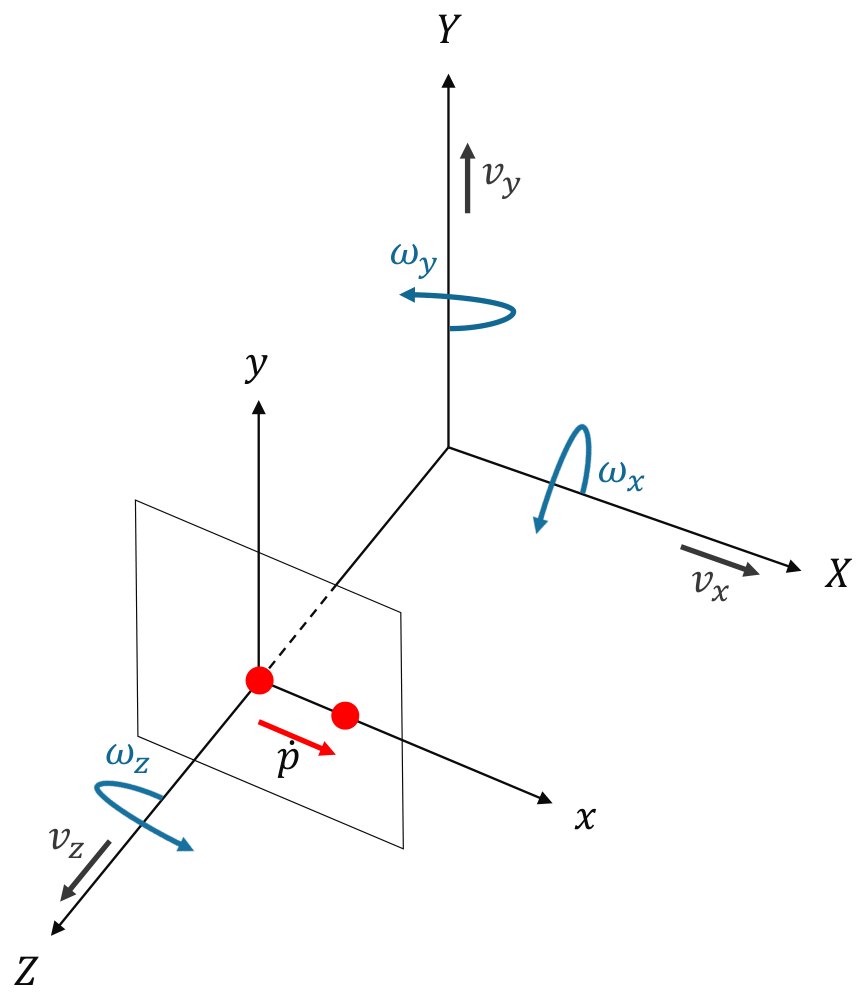
Assume a rigid, static scene and a camera with translational velocity $\mathbf{V} = [V_x, V_y, V_z]^T$ and rotational velocity $\boldsymbol{\Omega} = [\omega_x, \omega_y, \omega_z]^T$ . A scene point $\mathbf{P} = [X, Y, Z]^T$ , expressed in the camera frame, projects to the normalized image point $\mathbf{p} = [x, y, 1]^T$ :

x = \frac{X}{Z}, \qquad y = \frac{Y}{Z}, \qquad \mathbf{p} = \frac{1}{Z}\mathbf{P}

Camera coordinate axes X, Y and Z with translational velocities v and rotational velocities omega, and an image plane on which a point moves with velocity p-dot — Camera frame, image plane and the six components of camera motion.

Derivation

Step 1: Motion of the point. Relative to the camera, a static point moves opposite to the camera’s motion:

\dot{\mathbf{P}} = -\boldsymbol{\Omega} \times \mathbf{P} - \mathbf{V}

Expanding the cross product gives

\begin{aligned} \dot{X} &= -V_x - \omega_y Z + \omega_z Y \\ \dot{Y} &= -V_y - \omega_z X + \omega_x Z \\ \dot{Z} &= -V_z - \omega_x Y + \omega_y X \end{aligned}

Step 2: Differentiate the projection. Applying the quotient rule to $\mathbf{p} = \mathbf{P}/Z$ gives $\dot{\mathbf{p}} = \dot{\mathbf{P}}/Z - (\dot{Z}/Z)\,\mathbf{p}$ , or in components:

\dot{x} = \frac{\dot{X} - x\dot{Z}}{Z}, \qquad \dot{y} = \frac{\dot{Y} - y\dot{Z}}{Z}

Step 3: Substitute. Inserting the expressions from Step 1 and replacing $X/Z$ with $x$ and $Y/Z$ with $y$ gives

\begin{aligned} \dot{x} &= \frac{xV_z - V_x}{Z} + xy\,\omega_x - (1 + x^2)\,\omega_y + y\,\omega_z \\[6pt] \dot{y} &= \frac{yV_z - V_y}{Z} + (1 + y^2)\,\omega_x - xy\,\omega_y - x\,\omega_z \end{aligned}

In matrix form, this is the motion field equation:

\dot{\mathbf{p}} = \underbrace{\frac{1}{Z} \begin{bmatrix} xV_z - V_x \\ yV_z - V_y \end{bmatrix}}_{\text{translational flow}} + \underbrace{\begin{bmatrix} xy & -(1 + x^2) & y \\ (1 + y^2) & -xy & -x \end{bmatrix} \boldsymbol{\Omega}}_{\text{rotational flow}}

Translation and Rotation

The two components behave very differently:

Translational flow depends on depth. It scales with $1/Z$ , so nearby points move faster in the image. This effect is known as motion parallax.
Rotational flow is independent of depth. $Z$ does not appear in this term, so a purely rotating camera provides no information about scene structure.
Scale is ambiguous. Translation and depth appear only as the ratio $\mathbf{V}/Z$ , so a single camera cannot recover absolute scale from image motion alone.

Special Cases

Setting all but one velocity component to zero isolates the basic flow patterns. The animations below are computed directly from the motion field equation at constant depth, with image $x$ pointing right, image $y$ pointing down and $Z$ pointing forward. Reversing a velocity reverses its arrows.

Pure translation. Sideways motion gives uniform flow opposite to the camera, and forward motion gives radial flow:

V_x > 0

: camera moves right, flow is to the left.

V_y > 0

: camera moves down, flow is upward.

V_z > 0

: camera moves forward, flow expands.

Pure rotation. Rotation about $x$ or $y$ gives nearly uniform flow near the image center that curves toward the edges, and rotation about the optical axis gives circular flow:

\omega_x > 0

: camera tilts up, flow is downward.

\omega_y > 0

: camera pans right, flow is to the left.

\omega_z > 0

: camera rolls, flow circles the center.

Near the image center, rotation about $y$ and translation along $x$ look nearly identical: for small $x$ and $y$ , $\dot{x} \approx -\omega_y$ and $\dot{y} \approx 0$ . The same holds for rotation about $x$ and translation along $y$ , so the two are difficult to separate with a narrow field of view.

Inside the red box, a narrow field of view, the two motions produce almost the same flow.

Explore the Equation

The explorer below evaluates the motion field equation live. Choose a camera motion and a scene, then move the pointer over the image to read the flow at that point.

Scene Remove rotational flow

Image center: (0, 0)
Depth Z: 1.0
Flow: (0, 0)
FOE: (0, 0)
Time to contact: 1.7

Two experiments are worth trying. First, select Forward + pan: the rotation hides the direction of travel, and the flow appears to expand from the wrong place. Removing the rotational flow reveals the true FOE, which is why robots estimate and subtract rotation first, often with a gyroscope. Second, select Sideways with Two objects at different depths: the nearer object visibly moves faster, and that difference is the depth signal.

Focus of Expansion

Factoring $V_z$ out of the translational flow gives

\dot{\mathbf{p}}_{\text{trans}} = \frac{V_z}{Z} \begin{bmatrix} x - V_x/V_z \\ y - V_y/V_z \end{bmatrix}

This flow is zero at a single image point, and every flow vector points along the line through it. This point is the focus of expansion (FOE), and it marks the camera’s direction of travel:

\text{FOE} = \left(\frac{V_x}{V_z},\; \frac{V_y}{V_z}\right)

When $V_z = 0$ , the FOE moves to infinity and the flow vectors become parallel.

Time to Contact

The time to contact $\tau$ is the time remaining before the camera reaches the plane of a point, assuming constant velocity:

\tau = \frac{Z}{V_z}

Taking the magnitude of the translational flow above and rearranging gives

\tau = \frac{Z}{V_z} = \frac{\|\mathbf{p} - \text{FOE}\|}{\|\dot{\mathbf{p}}_{\text{trans}}\|}

Notably, time to contact can be measured from a single moving camera without knowing either depth or speed, even though neither can be recovered individually. It requires only the flow vector and its distance from the FOE. Among points at the same distance from the FOE, longer flow vectors therefore indicate a more imminent collision.

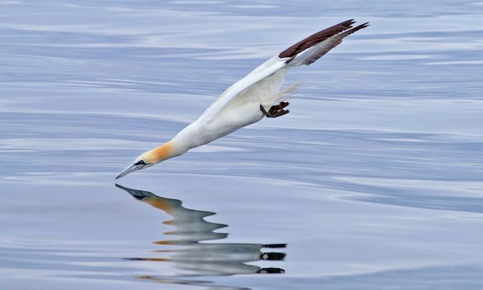
Time to contact is widely used for obstacle avoidance on small robots, and it also appears in nature. Gannets enter the sea like torpedoes: they plunge at high speed and must fold their wings just before impact. Their timing is consistent with a time-to-contact estimate from the expanding image of the water, rather than separate estimates of height and speed [1, 2].

A gannet with folded wings diving just above the water, its reflection visible on the surface — A gannet moments before entering the water, with its wings folded back.

Motion Field vs. Optical Flow

A camera cannot measure the motion field directly. It observes only changing brightness patterns, and the apparent motion of these patterns is called optical flow. Optical flow is an observable approximation of the motion field, but the two are not always equal.

Optical flow estimated from a traffic video, with color encoding the direction of motion.

A rotating sphere shows the difference. Both spheres below rotate, so both have the same motion field, but only the textured one produces optical flow. A uniform sphere looks unchanged.

Motion without flow: the motion field is the same for both spheres, but the uniform sphere has no optical flow.

The reverse also occurs. A moving light changes the shading across a stationary sphere and its surroundings, which produces optical flow although the motion field is zero.

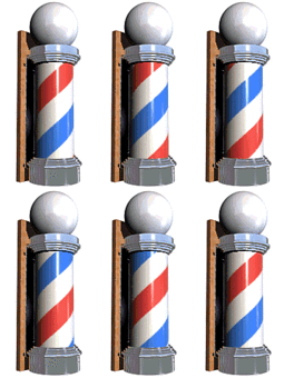
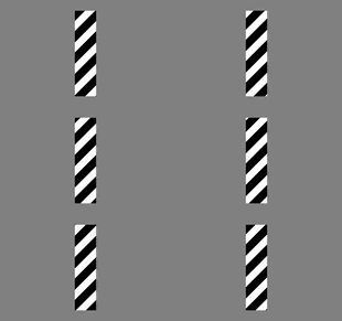
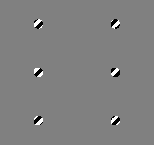
Flow without motion: the sphere is stationary, and only the light moves.

Local measurements add a further ambiguity. Through a small window, only the component of motion perpendicular to an edge can be observed. This is the aperture problem, and it explains why a barber pole’s stripes appear to move vertically although the pole rotates horizontally.

A rotating barber pole whose stripes appear to move upward — Barber pole: the motion field is horizontal, but the optical flow is vertical.

Diagonal stripes moving inside a tall narrow window — Stripes through a narrow window.

Diagonal stripes moving behind a small circular window — Stripes through a small aperture.

References

D. N. Lee, “A theory of visual control of braking based on information about time-to-collision,” Perception, 1976.
D. N. Lee and P. E. Reddish, “Plummeting gannets: a paradigm of ecological optics,” Nature, 1981.