ROBO/MCEN 5228: Advanced Computer Vision
Geometry and Learning-based Methods in Computer Vision
Project 3: Part 1 | Structure from Motion
Table of Contents
- Deadline
- Introduction
- Part 1: Structure From Motion
- 3.1. Feature Matching
- 3.2. Estimating Fundamental Matrix
- 3.2.1 Epipolar Geometry
- 3.2.2 Fundamental Matrix
- 3.2.3 RANSAC Outlier Rejection
- 3.3 Estimate Essential Matrix from Fundamental Matrix
- 3.4 Estimate Camera Pose from Essential Matrix
- 3.5 Check for Cheirality Condition using Triangulation
- 3.5.1 Non-Linear Triangulation
- 3.6 Perspective-n-points
- 3.6.1 Linear Camera Pose Estimation
- 3.6.2 PnP RANSAC
- 3.6.3 NonLinear PnP
- 3.7 Bundle Adjustment
- 3.7.1 Visibility Matrix
- 3.7.2 Bundle Adjustment Optimization
- Putting the pipeline together
- Notes about Data Set
- Submission Guidelines
- 6.1. File tree and naming
- 6.2. Report
- Collaboration Policy
1. Deadline
- 3.1. Feature Matching
- 3.2. Estimating Fundamental Matrix
- 3.2.1 Epipolar Geometry
- 3.2.2 Fundamental Matrix
- 3.2.3 RANSAC Outlier Rejection
- 3.3 Estimate Essential Matrix from Fundamental Matrix
- 3.4 Estimate Camera Pose from Essential Matrix
- 3.5 Check for Cheirality Condition using Triangulation
- 3.5.1 Non-Linear Triangulation
- 3.6 Perspective-n-points
- 3.6.1 Linear Camera Pose Estimation
- 3.6.2 PnP RANSAC
- 3.6.3 NonLinear PnP
- 3.7 Bundle Adjustment
- 3.7.1 Visibility Matrix
- 3.7.2 Bundle Adjustment Optimization
- 6.1. File tree and naming
- 6.2. Report
11:59PM, Nov 27, 2024. To be submitted with Part 2 (Gaussian Splatting) in a group of 2.
2. Introduction
We have been playing with images for so long, mostly in 2D scenes. Recall Panorama project where we stitched multiple images with about 30-50% common features between a couple of images. Now let's learn how to reconstruct a 3D scene and simultaneously obtain the camera poses of a monocular camera w.r.t. the given scene. This procedure is known as Structure from Motion (SfM). As the name suggests, you are creating the entire rigid structure from a set of images with different viewpoints (or equivalently a camera in motion). A few years ago, Agarwal et al. published Building Rome in a Day, in which they reconstructed the entire city just by using a large collection of photos from the Internet. Ever heard of Microsoft Photosynth? Fascinating, isn't it!? There are a few open-source SfM algorithms available online like VisualSFM. Another open source SfM pipeline with GUI is COLMAP! Try them out!
Let's learn how to recreate such an algorithm. There are a few steps that collectively form SfM:
- Feature Matching and Outlier rejection using RANSAC
- Estimating Fundamental Matrix
- Estimating Essential Matrix from Fundamental Matrix
- Estimate Camera Pose from Essential Matrix
- Check for Cheirality Condition using Triangulation
- Perspective-n-Point
- Bundle Adjustment
3. Traditional Approach to the SfM Problem
3.1. Feature Matching, Fundamental Matrix, and RANSAC
We have already learned about keypoint matching using SIFT keypoints and descriptors (Recall Project 1: Panorama Stitching). It is important to refine the matches by rejecting outlier correspondences. Before rejecting the correspondences, let us first understand what the Fundamental matrix is!
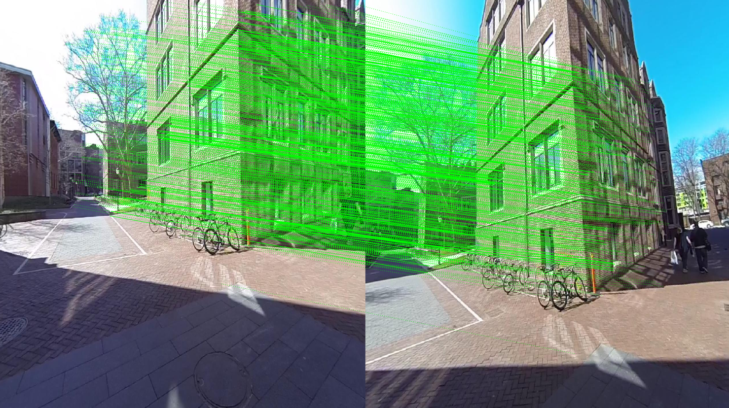
Figure 1: Feature matching between two images from different views.
3.2. Estimating Fundamental Matrix
The fundamental matrix, denoted by \( \mathbf{F} \), is a \( 3 \times 3 \) (rank 2) matrix that relates the corresponding set of points in two images from different views (or stereo images). But in order to understand what the fundamental matrix actually is, we need to understand what epipolar geometry is! The epipolar geometry is the intrinsic projective geometry between two views. It only depends on the cameras' internal parameters (denoted by the \( \mathbf{K} \) matrix) and the relative pose, i.e., it is independent of the scene structure.
3.2.1. Epipolar Geometry
Let's say a point \( \mathbf{X} \) in the 3D-space (viewed in two images) is captured as \( \mathbf{x} \) in the first image and \( \mathbf{x'} \) in the second. Can you think how to formulate the relation between the corresponding image points \( \mathbf{x} \) and \( \mathbf{x'} \)? Consider Fig. 2. Let \( \mathbf{C} \) and \( \mathbf{C'} \) be the respective camera centers, which form the baseline for the stereo system. Clearly, the points \( \mathbf{x} \), \( \mathbf{x'} \), and \( \mathbf{X} \) (or \( \mathbf{C} \), \( \mathbf{C'} \), and \( \mathbf{X} \)) are coplanar, i.e.: \[ \mathbf{\overrightarrow{Cx}} \cdot \left( \mathbf{\overrightarrow{CC'}} \times \mathbf{\overrightarrow{C'x'}} \right) = 0 \] The plane formed can be denoted by \( \pi \). Since these points are coplanar, the rays back-projected from \( \mathbf{x} \) and \( \mathbf{x'} \) intersect at \( \mathbf{X} \). This is the most significant property in searching for a correspondence.
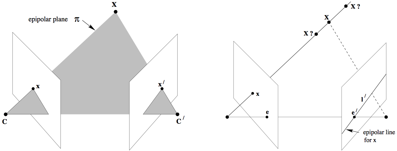
Figure 2(a): Epipolar planes and epipolar lines
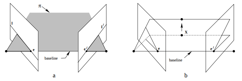
Figure 2(b): Baseline joining two camera centers lying on the epipolar plane
Now, let us say that only \( \mathbf{x} \) is known, not \( \mathbf{x'} \). We know that the point \( \mathbf{x'} \) lies in the plane \( \pi \) which is governed by the camera baseline \( \mathbf{CC'} \) and \( \mathbf{\overrightarrow{Cx}} \). Hence the point \( \mathbf{x'} \) lies on the line of intersection \( \mathbf{l'} \) of \( \pi \) with the second image plane. The line \( \mathbf{l'} \) is the image in the second view of the ray back-projected from \( \mathbf{x} \). This line \( \mathbf{l'} \) is called the epipolar line corresponding to \( \mathbf{x} \). The benefit is that you don't need to search for the point corresponding to \( \mathbf{x} \) in the entire image plane as it can be restricted to \( \mathbf{l'} \).
- Epipole is the point of intersection of the line joining the camera centers with the image plane. (see \( \mathbf{e} \) and \( \mathbf{e'} \) in Fig. 2(a))
- Epipolar plane is the plane containing the baseline.
- Epipolar line is the intersection of an epipolar plane with the image plane. All the epipolar lines intersect at the epipole.
3.2.2. The Fundamental Matrix \( \mathbf{F} \)
The \( \mathbf{F} \) matrix is only an algebraic representation of epipolar geometry and can be derived both geometrically (constructing the epipolar line) and arithmetically. (See derivation (Page 242)) (Fundamental Matrix Song)
As a result, we obtain: \[ \mathbf{x}_i'^{\ \mathbf{T}}\mathbf{F} \mathbf{x}_i = 0 \] where \( i = 1, 2, \ldots, m \). This is known as the epipolar constraint or correspondence condition (also known as the Longuet-Higgins equation). Since \( \mathbf{F} \) is a \( 3 \times 3 \) matrix, we can set up a homogeneous linear system with 9 unknowns:
\[ \begin{bmatrix} x'_i & y'_i & 1 \end{bmatrix} \begin{bmatrix} f_{11} & f_{12} & f_{13} \\ f_{21} & f_{22} & f_{23} \\ f_{31} & f_{32} & f_{33} \end{bmatrix} \begin{bmatrix} x_i \\ y_i \\ 1 \end{bmatrix} = 0 \]\[ x_i x'_i f_{11} + x_i y'_i f_{21} + x_i f_{31} + y_i x'_i f_{12} + y_i y'_i f_{22} + y_i f_{32} + x'_i f_{13} + y'_i f_{23} + f_{33} = 0 \]
Simplifying for \( m \) correspondences,
\[ \begin{bmatrix} x_1 x'_1 & x_1 y'_1 & x_1 & y_1 x'_1 & y_1 y'_1 & y_1 & x'_1 & y'_1 & 1 \\ \vdots & \vdots & \vdots & \vdots & \vdots & \vdots & \vdots & \vdots & \vdots \\ x_m x'_m & x_m y'_m & x_m & y_m x'_m & y_m y'_m & y_m & x'_m & y'_m & 1 \end{bmatrix} \begin{bmatrix} f_{11} \\ f_{21} \\ f_{31} \\ f_{12} \\ f_{22} \\ f_{32} \\ f_{13} \\ f_{23} \\ f_{33} \end{bmatrix} = 0 \]How many points do we need to solve the above equation? Think! Twice! Remember homography, where each point correspondence contributes two constraints? Unlike homography, in \( \mathbf{F} \) matrix estimation, each point only contributes one constraint as the epipolar constraint is a scalar equation. Thus, we require at least 8 points to solve the above homogeneous system. That is why it is known as the Eight-point algorithm.
With \( N \geq 8 \) correspondences between two images, the fundamental matrix, \( F \) can be obtained as:
By stacking the above equation in a matrix \( A \), the equation \( Ax = 0 \) is obtained. This system of equations can be solved by minimizing the linear least squares using Singular Value Decomposition (SVD), as explained in the Math module. When applying SVD to matrix \( \mathbf{A} \), the decomposition \( \mathbf{USV}^T \) would be obtained, where \( \mathbf{U} \) and \( \mathbf{V} \) are orthonormal matrices, and \( \mathbf{S} \) is a diagonal matrix containing the singular values. The singular values \( \sigma_i \) where \( i \in [1,9], i \in \mathbb{Z} \), are positive and are in decreasing order with \( \sigma_9 = 0 \) since we have 8 equations for 9 unknowns. Thus, the last column of \( \mathbf{V} \) is the true solution, given that \( \sigma_i \neq 0 \ \forall i \in [1,8], i \in \mathbb{Z} \).
However, due to noise in the correspondences, the estimated \( \mathbf{F} \) matrix can be of rank 3, i.e. \( \sigma_9 \neq 0 \). To enforce the rank 2 constraint, the last singular value of the estimated \( \mathbf{F} \) must be set to zero. If \( F \) has full rank, then it will have an empty null-space, i.e., it won't have any point that is on the entire set of lines. Thus, there wouldn't be any epipoles. See Fig. 3 for full rank comparisons for \( F \) matrices.
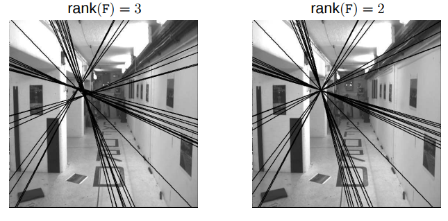
Figure 3: F Matrix: Rank 3 vs Rank 2 comparison
In Python, you can use np.linalg.svd to solve \( \mathbf{x} \) from \( \mathbf{Ax} = 0 \)
  U, S, Vt = np.linalg.svd(A)
  x = Vt[-1, :]    # Last row of V transpose gives the solution vector
  F = x.reshape((3, 3)).T # Reshape and transpose to construct F matrix
To summarize, write a function EstimateFundamentalMatrix.py that linearly estimates a fundamental matrix \( F \), such that \( x_2^T F x_1 = 0 \). The fundamental matrix can be estimated by solving the linear least squares \( Ax = 0 \).
3.2.3. Match Outlier Rejection via RANSAC
Since the point correspondences are computed using SIFT or some other feature descriptors, the data is bound to be noisy and (in general) contains several outliers. Thus, to remove these outliers, we use the RANSAC algorithm (Yes! The same as used in Panorama stitching!) to obtain a better estimate of the fundamental matrix. So, out of all possibilities, the \( \mathbf{F} \) matrix with the maximum number of inliers is chosen.
Below is the pseudo-code that returns the \( \mathbf{F} \) matrix for a set of matching corresponding points (computed using SIFT) which maximizes the number of inliers.
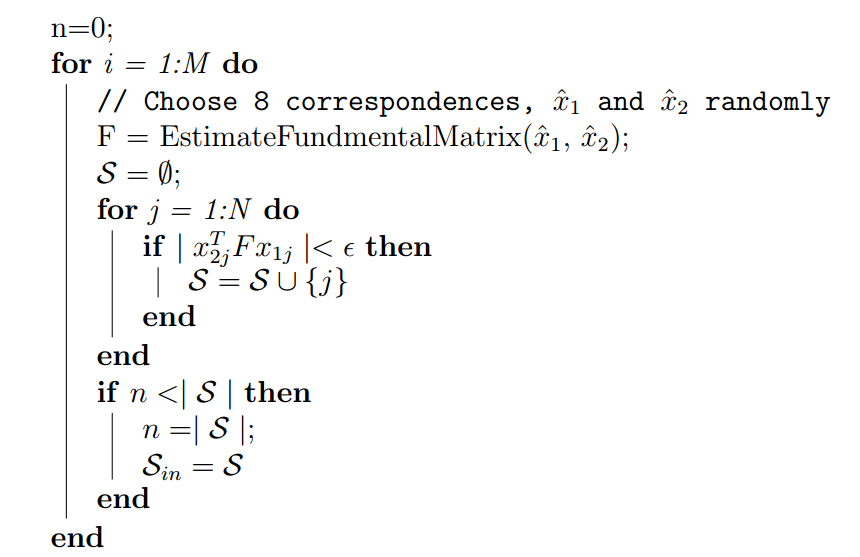
Algorithm 1: Get Inliers RANSAC
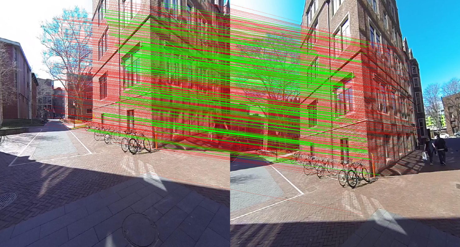
Figure 4: Feature matching after RANSAC. (Green: Selected correspondences; Red: Rejected correspondences)
Given, \( N \geq 8 \) correspondences between two images, \( x_1 \leftrightarrow x_2 \), implement a function GetInlierRANSAC.py that estimates inlier correspondences using fundamental matrix-based RANSAC.
3.3. Estimate Essential Matrix from Fundamental Matrix
Since we have computed the \( \mathbf{F} \) using epipolar constraints, we can find the relative camera poses between the two images. This can be computed using the Essential Matrix, \( \mathbf{E} \). The essential matrix is another \( 3 \times 3 \) matrix, but with some additional properties that relate the corresponding points, assuming that the cameras obey the pinhole model (unlike \( \mathbf{F} \)). More specifically,
\[ \mathbf{E} = \mathbf{K}^\mathbf{T} \mathbf{F} \mathbf{K} \]where \( \mathbf{K} \) is the camera calibration matrix or camera intrinsic matrix. Clearly, the essential matrix can be extracted from \( \mathbf{F} \) and \( \mathbf{K} \). As in the case of \( \mathbf{F} \) matrix computation, the singular values of \( \mathbf{E} \) are not necessarily \( (1, 1, 0) \) due to noise in \( \mathbf{K} \). This can be corrected by reconstructing it with \( (1, 1, 0) \) singular values, i.e.
\[ \mathbf{E} = U \begin{bmatrix} 1 & 0 & 0 \\ 0 & 1 & 0 \\ 0 & 0 & 0 \end{bmatrix} V^\mathbf{T} \]It is important to note that \( \mathbf{F} \) is defined in the original image space (i.e., pixel coordinates), whereas \( \mathbf{E} \) is in the normalized image coordinates. Normalized image coordinates have the origin at the optical center of the image. Also, relative camera poses between two views can be computed using the \( \mathbf{E} \) matrix. Moreover, \( \mathbf{F} \) has 7 degrees of freedom while \( \mathbf{E} \) has 5 as it takes camera parameters into account. (5-Point Motion Estimation Made Easy)
Given \( F \), estimate the essential matrix \( E = K^\mathbf{T} F K \) by implementing the function EssentialMatrixFromFundamentalMatrix.py.
3.4. Estimate Camera Pose from Essential Matrix
The camera pose consists of 6 degrees-of-freedom (DOF): Rotation (Roll, Pitch, Yaw) and Translation (X, Y, Z) of the camera with respect to the world. Since the \( \mathbf{E} \) matrix is identified, the four camera pose configurations: \( (C_1, R_1) \), \( (C_2, R_2) \), \( (C_3, R_3) \), and \( (C_4, R_4) \), where \( C \in \mathbb{R}^3 \) is the camera center and \( R \in SO(3) \) is the rotation matrix, can be computed. Thus, the camera pose can be written as:
\[ P = K R \begin{bmatrix} I_{3 \times 3} & -C \end{bmatrix} \]These four pose configurations can be computed from the \( \mathbf{E} \) matrix. Let \( \mathbf{E} = UDV^T \) and \( W = \begin{bmatrix} 0 & -1 & 0 \\ 1 & 0 & 0 \\ 0 & 0 & 1 \end{bmatrix} \). The four configurations can be written as:
- \( C_1 = U(:, 3) \) and \( R_1 = UWV^T \)
- \( C_2 = -U(:, 3) \) and \( R_2 = UWV^T \)
- \( C_3 = U(:, 3) \) and \( R_3 = UW^TV^T \)
- \( C_4 = -U(:, 3) \) and \( R_4 = UW^TV^T \)
It is important to note that \( \det(R) = 1 \). If \( \det(R) = -1 \), the camera pose must be corrected, i.e., \( C = -C \) and \( R = -R \). Implement the function ExtractCameraPose.py, given \( E \).
3.5. Triangulation Check for Cheirality Condition
In the previous section, we computed four different possible camera poses for a pair of images using the essential matrix. In this section, we will triangulate the 3D points, given two camera poses.
Given two camera poses, \( (C_1, R_1) \) and \( (C_2, R_2) \), and correspondences, \( x_1 \leftrightarrow x_2 \), triangulate 3D points using linear least squares. Implement the function LinearTriangulation.py.
However, to find the correct unique camera pose, we need to resolve the ambiguity. This can be accomplished by checking the cheirality condition, i.e., the reconstructed points must be in front of the cameras.
To check the cheirality condition, triangulate the 3D points (given two camera poses) using linear least squares to verify the sign of the depth \( Z \) in the camera coordinate system with respect to the camera center. A 3D point \( X \) is in front of the camera if and only if:
\[ r_3 \cdot (\mathbf{X} - \mathbf{C}) > 0 \]where \( r_3 \) is the third row of the rotation matrix (z-axis of the camera). Not all triangulated points satisfy this condition due to the presence of correspondence noise. The best camera configuration, \( (C, R, X) \), is the one that produces the maximum number of points satisfying the cheirality condition.
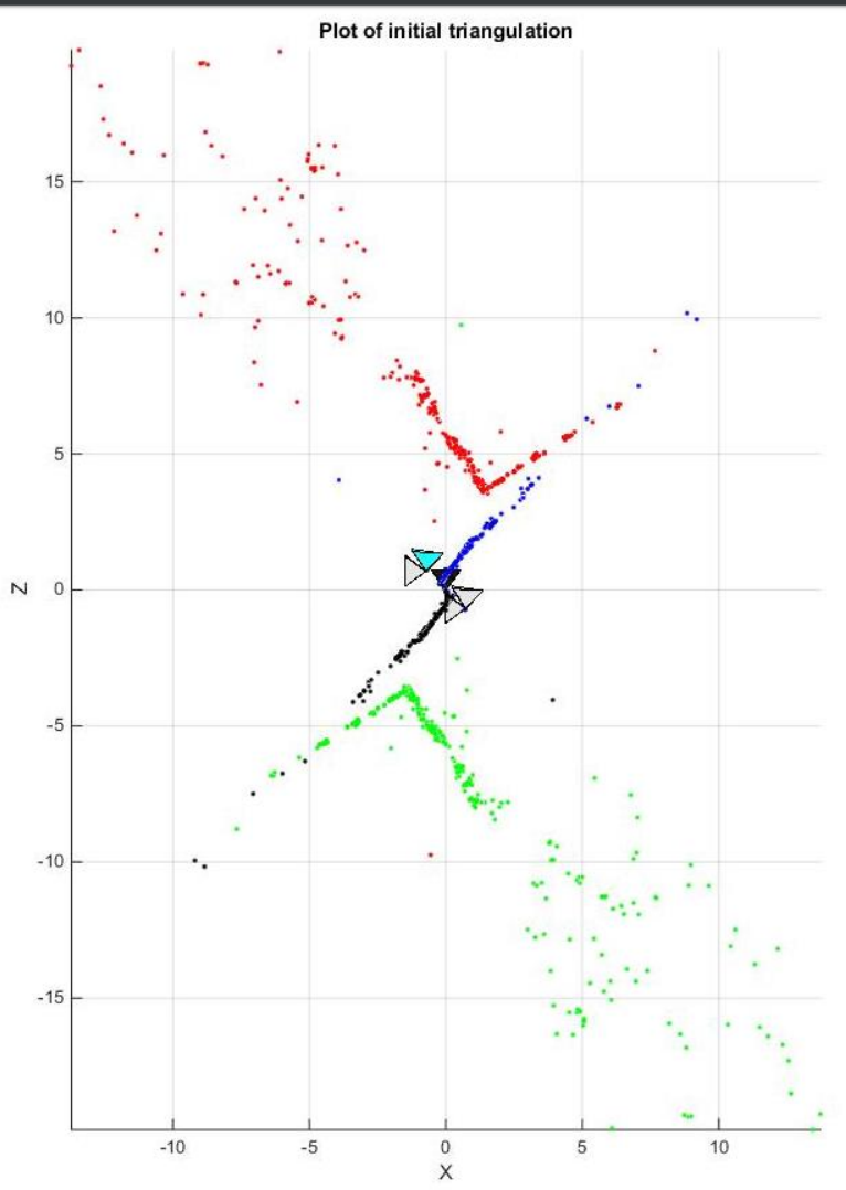
Figure 5: Initial triangulation plot with ambiguity, showing all four possible camera poses.
Given four camera pose configurations and their triangulated points, find the unique camera pose by checking the cheirality condition – the reconstructed points must be in front of the cameras (implement the function DisambiguateCameraPose.py).
3.5.1. Non-Linear Triangulation
Given two camera poses and linearly triangulated points, \( X \), the locations of the 3D points that minimize the reprojection error (Recall Project 2) can be refined. The linear triangulation minimizes the algebraic error. However, the reprojection error is a geometrically meaningful error and can be computed by measuring the error between the measurement and the projected 3D point:
\[ \underset{x}{\operatorname{min}} \sum_{j=1,2} \left( u^j - \frac{P_1^{jT} \widetilde{X}}{P_3^{jT} X} \right)^2 + \left( v^j - \frac{P_2^{jT} \widetilde{X}}{P_3^{jT} X} \right)^2 \]Here, \( j \) is the index of each camera, \( \widetilde{X} \) is the homogeneous representation of \( X \). \( P_i^T \) is each row of the camera projection matrix, \( P \). This minimization is highly nonlinear due to the divisions. The initial guess of the solution, \( X_0 \), is estimated via linear triangulation to minimize the cost function. This minimization can be solved using nonlinear optimization functions such as scipy.optimize.leastsq or scipy.optimize.least_squares in the SciPy library.
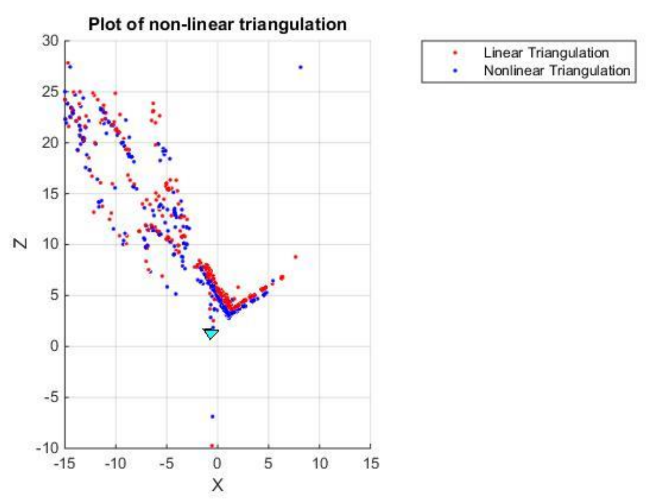
Figure 6: Comparison between non-linear vs linear triangulation.
Given two camera poses and linearly triangulated points, \( X \), refine the locations of the 3D points that minimize the reprojection error (implement the function NonlinearTriangulation.py).
3.6. Perspective-\(n\)-Points
Now, since we have a set of \( n \) 3D points in the world, their 2D projections in the image, and the intrinsic parameter, the 6 DOF camera pose can be estimated using linear least squares. This fundamental problem is generally known as Perspective-\( n \)-Point (PnP). For there to exist a solution, \( n \geq 3.\) There are multiple methods to solve the P\( n \)P problem, and most of them assume that the camera is calibrated. Methods such as Unified P\( n \)P (or UPnP) do not adhere to this assumption, as they estimate both intrinsic and extrinsic parameters. In this section, you will explore a simpler version of PnP. You will register a new image given 2D-3D correspondences, i.e., \( X \leftrightarrow x \), followed by nonlinear optimization.
3.6.1 Linear Camera Pose Estimation
Given 2D-3D correspondences, \( X \leftrightarrow x \), and the intrinsic parameter \( K \), estimate the camera pose using linear least squares (implement the function LinearPnP.py). 2D points can be normalized by the intrinsic parameter to isolate camera parameters, \( (C, R) \), i.e., \( K^{-1} x \). A linear least squares system that relates the 3D and 2D points can be solved for \( (t, R) \) where \( t = -R^T C \). Since the linear least square solution does not enforce orthogonality of the rotation matrix, \( R \in SO(3) \), the rotation matrix must be corrected by \( R = UV^T \) where \( R = UDV^T \). If the corrected rotation has a determinant of \( -1 \), then \( R = -R \). This linear PnP requires at least 6 correspondences. (Think why?)
Figure 7: Plot of the camera poses with feature points. Different colors represent feature correspondences from different pairs of images. Blue points are features from Image 1 and Image 2; Red points are features from Image 2 and Image 3, etc.
3.6.2 PnP RANSAC
PnP is prone to error as there are outliers in the given set of point correspondences. To overcome this error, we can use RANSAC (yes, again!) to make our camera pose estimation more robust to outliers. To formalize, given \( N \geq 6 \) 3D-2D correspondences, \( X \leftrightarrow x \), implement the following function that estimates the camera pose \( (C, R) \) via RANSAC (implement the function PnPRANSAC.py).
The algorithm below depicts the solution using RANSAC.

Algorithm 2: PnP RANSAC
Just like in triangulation, since we have the linearly estimated camera pose, we can refine the camera pose to minimize the reprojection error (Linear PnP only minimizes the algebraic error).
3.6.3 Nonlinear PnP
Given \( N \geq 6 \) 3D-2D correspondences, \( X \leftrightarrow x \), and a linearly estimated camera pose, \( (C, R) \), refine the camera pose to minimize the reprojection error (implement the function NonlinearPnP.py). The linear PnP minimizes algebraic error. The reprojection error, a geometrically meaningful error, is computed by measuring the error between the measurement and the projected 3D point:
Here, \( \widetilde{X} \) is the homogeneous representation of \( X \). \( P_i^T \) represents each row of the camera projection matrix, \( P \), which is computed as \( P = K R [I_{3 \times 3} - C] \). A compact representation of the rotation matrix using a quaternion is a better choice to enforce orthogonality of the rotation matrix, \( R = R(q) \), where \( q \) is a four-dimensional quaternion. Thus, we have:
\[ \underset{C, q}{\operatorname{min}} \sum_{j=1}^{J} \left( u^j - \frac{P_1^{jT} \widetilde{X_j}}{P_3^{jT} \widetilde{X_j}} \right)^2 + \left( v^j - \frac{P_2^{jT} \widetilde{X_j}}{P_3^{jT} \widetilde{X_j}} \right)^2 \]This minimization is highly nonlinear due to the divisions and quaternion parameterization. The initial guess of the solution, \( (C_0, R_0) \), estimated via linear PnP, is needed to minimize the cost function. This minimization can be solved using a nonlinear optimization function such as scipy.optimize.leastsq or scipy.optimize.least_squares in the SciPy library.
3.7. Bundle Adjustment
Once you have computed all the camera poses and 3D points, we need to refine the poses and 3D points together, initialized by the previous reconstruction, by minimizing the reprojection error.
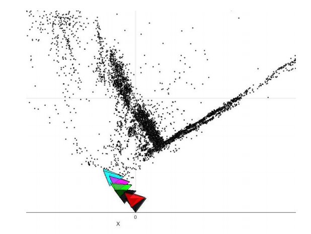
Figure 7: The final reconstructed scene after Sparse Bundle Adjustment (SBA).
3.7.1 Visibility Matrix
Find the relationship between a camera and point, and construct an \( I \times J \) binary matrix, \( V \), where \( V_{ij} \) is one if the \( j^{th} \) point is visible from the \( i^{th} \) camera and zero otherwise (implement the function BuildVisibilityMatrix.py).
3.7.2 Bundle Adjustment Optimization
Given initialized camera poses and 3D points, refine them by minimizing the reprojection error (implement the function BundleAdjustment.py). Bundle adjustment refines camera poses and 3D points simultaneously by minimizing the following reprojection error over \( C_{i_{i=1}}^I \), \( q_{i_{i=1}}^I \), and \( X_{j_{j=1}}^J \).
The optimization problem can be formulated as follows:
\[ \underset{\{C_i, q_i\}_{i=1}^I, \{X\}_{j=1}^J}{\operatorname{min}} \sum_{i=1}^I \sum_{j=1}^J V_{ij} \left( \left( u^j - \frac{P_1^{jT} \tilde{X}}{P_3^{jT} \tilde{X}} \right)^2 + \left( v^j - \frac{P_2^{jT} \tilde{X}}{P_3^{jT} \tilde{X}} \right)^2 \right) \]where \( V_{ij} \) is the visibility matrix.
Clearly, solving such a method to compute the structure from motion is complex and slow (can take from several minutes for only 8-10 images). This minimization can be solved using nonlinear optimization functions such as scipy.optimize.leastsq, but will be extremely slow due to the number of parameters. Sparse Bundle Adjustment toolboxes, such as pySBA and large-scale BA in scipy, are designed to solve such optimization by exploiting the sparsity of the visibility matrix, \( V \). Note that a small number of entries in \( V \) are one because a 3D point is visible from a small subset of images. Using the sparse bundle adjustment package is not trivial but would be much faster than one you write. For SBA, you are allowed to use any optimization library.
4. Putting the pipeline together
Write a program Wrapper.py that runs the full pipeline of structure from motion based on the above algorithm.
Also, compare your result against COLMAP or VSfM output.
Project Overview
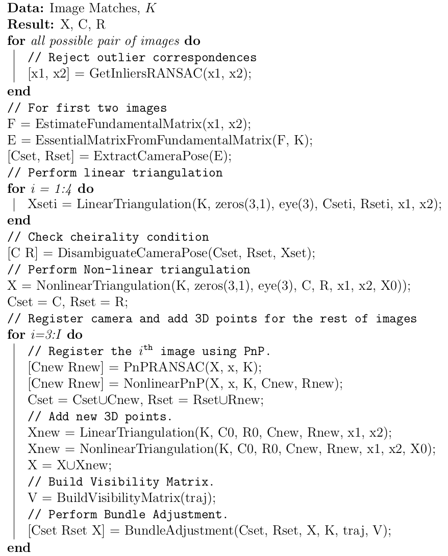
Figure 8: The overview.
5. Notes about the Sample Data
Run your SfM algorithm on the images provided here. The data given to you consists of a set of 6 images of a building in front of Levine Hall at UPenn, captured using a GoPro Hero 3 with fisheye lens distortion corrected. Keypoint matching (SIFT keypoints and descriptors) data is also provided in the same folder for pairs of images. The data folder contains 5 matching files named matching*.txt, where * refers to numbers from 1 to 5. For example, matching3.txt contains the matching between the third image and the fourth, fifth, and sixth images, i.e., \( \mathcal{I}_3 \leftrightarrow \mathcal{I}_4 \), \( \mathcal{I}_3 \leftrightarrow \mathcal{I}_5 \), and \( \mathcal{I}_3 \leftrightarrow \mathcal{I}_6 \). Therefore, matching6.txt does not exist because it would represent a match of the image with itself.
The format of the matching files is described below. Each matching file is formatted as follows for the \( i^{th} \) matching file:
- nFeatures: the number of feature points of the \( i^{th} \) image - each following row specifies matches across images for a feature location in the \( i^{th} \) image.
- Each Row: (the number of matches for the \( j^{th} \) feature) (Red Value) (Green Value) (Blue Value) \( u_{\texttt{current image}} \) \( v_{\texttt{current image}} \) (image id) \( u_{\texttt{image id image}} \) \( v_{\texttt{image id image}} \) ...
An example of matching1.txt is given below:
nFeatures: 2002
3 137 128 105 454.740000 392.370000 2 308.570000 500.320000 4 447.580000 479.360000
2 137 128 105 454.740000 392.370000 4 447.580000 479.360000
The images are taken at 1280 × 960 resolution, and the camera intrinsic parameters \( K \) are provided in the calibration.txt file. You will implement this full pipeline guided by the functions described in the following sections.
6. Submission Guidelines
Download the Starter Code and Data from here.
6.1. File Tree and Naming
Your submission on ELMS/Canvas must be a zip file, following the naming convention YourDirectoryID_p3.zip. If your email ID is abc@colorado.edu, then your DirectoryID is abc. For our example, the submission file should be named abc_p1.zip. The file must have the following directory structure because we will be autograding assignments. The file to run for your project should be called Wrapper.py. You may include helper functions in subfolders as needed; ensure you use relative paths and include default values for command line arguments in Wrapper.py. Please provide detailed instructions for running your code in the README.md file.
YourDirectoryID_p3.zip
│   README.md
|   Code/
|   ├── GetInliersRANSAC.py
|   ├── EstimateFundamentalMatrix.py
|   ├── EssentialMatrixFromFundamentalMatrix.py
|   ├── ExtractCameraPose.py
|   ├── LinearTriangulation.py
|   ├── DisambiguateCameraPose.py
|   ├── NonlinearTriangulation.py
|   ├── PnPRANSAC.py
|   ├── NonlinearPnP.py
|   ├── BuildVisibilityMatrix.py
|   ├── BundleAdjustment.py
|   ├── Wrapper.py
|   ├── Any subfolders you want along with files
|   ├── Wrapper.py
|   Data/
|   ├── BundleAdjustmentOutputForAllImage/
|   ├── FeatureCorrespondenceOutputForAllImageSet/
|   ├── LinearTriangulationOutputForAllImageSet/
|   ├── NonLinearTriangulationOutputForAllImageSet/
|   ├── PnPOutputForAllImageSetShowingCameraPoses/
|   ├── Imgs/
└── Report.pdf
6.2. Report
The final dataset for this project will release one week after the release. For each section of the project, explain briefly what you did, and describe any interesting problems you encountered and/or solutions you implemented. You must include the following details in your writeup:
- Make your report extremely detailed with reprojection error after each step (Linear, Non-linear triangulation, Linear, Non-linear PnP before and after BA, etc.). Describe all the steps (anything that is not obvious) and any other observations in your report.
- Your report MUST be typeset in LaTeX in the IEEE Tran format provided in the
Draftfolder and should be of conference-quality paper. - Present the data you collected in
Data/Imgs/. - Present failure cases and explanations, if any.
- Do not use any function that directly implements a part of the pipeline. If you have any doubts, please contact us via Piazza.
This project is derived from UMD's CMSC733 and Upenn's CIS580 course.